The Ultimate 2000’s Dance Party Playlist

Author

Vibha Gokhale

🎵 Hips Don’t Lie and We’re Dancing Like It’s 2005 🎵

Hips don’t lie and neither do these bangers from The Ultimate 2000s Dance Party Playlist. This playlist is The Ultimate because it brings together party classics, pop anthems, and Latin beats designed to maximize danceability, energy, and pure fun. With a mix of superhit songs like “Hips Don’t Lie” and “Smack That”, and some less popular gems like “Virtual Diva” and “Ella”, this playlist will keep you moving and grooving from start to finish.

Design Principles

The playlist is based on Spotify’s Song Characteristics and Million Playlists datasets. I analyzed tracks across key metrics and followed these guiding principles:

Danceability: I prioritized tracks with high danceability scores.
Energy and Tempo: Songs were ordered using energy, tempo, and valence trends. I chose songs with high energy and tempos above 95 BPM to maintain a consistent momentum and upbeat vibe.
Theme: I focused on tracks released between 2000 and 2010 to capture the dance-pop and Latin-infused sounds of the era.
Popularity Mix: I tried to balance recognizable hits with lesser-known tracks to sustain interest.

Warning: spontaneous dancing is basically guaranteed.💃

Appendix: Methodology

The following sections outline the steps used to create the “Ultimate Playlist.” Two data exports from Spotify were analyzed to identify the most popular songs and their characteristics.

Data Acquisition

Song Characteristics

Data about song characteristics was obtained from a mirror of the original Spotify data posted by GitHub user gabminamendez. The code below shows the process of downloading, importing, and cleaning this data.

Code

# load packages
library(tidyverse)
library(knitr)
library(kableExtra)
library(lubridate)
library(jsonlite)
library(purrr) 
library(scales)

# write load_songs function to get songs and their characteristics
load_songs <- function() {
  
  # set up the directory and file path
  dir_path <- "data/mp03"
  file_name <- "data.csv"
  file_path <- file.path(dir_path, file_name)
  file_url <- "https://raw.githubusercontent.com/gabminamedez/spotify-data/refs/heads/master/data.csv"

  # create directory if it doesn't exist
  if (!dir.exists(dir_path)) {
    dir.create(dir_path, showWarnings=FALSE, recursive = TRUE)
  }

  # download the file if it doesn't already exist
  if (!file.exists(file_path)) {
    download.file(file_url, destfile = file_path, method = "auto")
    }

  # read csv 
  songs <- read_csv(file_path, show_col_types = FALSE)
  
  # instructor code for cleaning 'artists' column
  clean_artist_string <- function(x){
    x |>
    str_replace_all("\\['", "") |>
    str_replace_all("'\\]", "") |>
    str_replace_all("[ ]?'", "") |>
    str_replace_all("[ ]*,[ ]*", ",") 
  }
  
  # cleaned songs data: one row per artist-track
  long_songs <- songs |> 
    separate_longer_delim(artists, ",") |>
    mutate(artist = clean_artist_string(artists)) |>
    select(-artists)
  
  # return data frame
  return(long_songs)
  }

# run function
long_songs <- load_songs()

# create a short version of cleaned songs data with one row per track
# all artists combined into one string; create 'number of artists' column
short_songs <- long_songs |>
  group_by(id) |>
  summarise(
    num_artists = n_distinct(artist),
    artist = paste(unique(artist), collapse = ", "),
    across(-artist,first),
    .groups = "drop")

The Song Characteristics dataset contains 169,909 distinct tracks from various artists and genres, released between 1921 and 2020. The data includes information about each track’s name, artist(s), duration, release date, as well as features such as acousticness, danceability, energy, instrumentalness, liveness, loudness, speechiness, tempo, valence, mode, key, popularity, and whether a track is explicit. I added a ‘number of artists’ column to indicate how many artists created a particular song. The table below shows a sample of the song characteristics data.

Code

# provide glimpse and summary of the shorter songs data only in interactive rstudio session
if (interactive()){
  glimpse(short_songs)
  summary(short_songs)}

# show a sample of song characteristics data
short_songs |> 
  slice_sample(n = 5) |>
  kbl(caption = "Sample of Song Characteristics Data") |> 
  kable_styling(bootstrap_options = c("striped", "hover")) |>
  scroll_box(width = "100%", height = "300px")

Sample of Song Characteristics Data
id	num_artists	artist	name	duration_ms	release_date	year	acousticness	danceability	energy	instrumentalness	liveness	loudness	speechiness	tempo	valence	mode	key	popularity
0oSCLH7cLuvCF4LXFRrWOs	1	Nick Cave & The Bad Seeds	Brother, My Cup Is Empty - 2010 Remastered Version	182493	1992	1992	0.0877	0.549	0.724	0.000	0.488	-6.810	0.0424	103.015	0.922	1	2	43
2zU14PbSlUxOfz2DWaeYHU	1	Fleetwood Mac	Go Your Own Way - Live 1977	294467	2/4/77	1977	0.0302	0.511	0.883	0.168	0.929	-8.010	0.0577	135.614	0.553	1	5	23
4owCqbb2fYTAYgtM6jjXIi	2	Dean Martin, Dick Stabile And His Orchestra	I'm Gonna Steal You Away - Remastered	152200	1957	1957	0.9450	0.726	0.142	0.000	0.166	-14.832	0.0488	100.465	0.668	0	7	12
07OgwcoS54OZgpUyehHhvM	2	Oscar Peterson Trio, Clark Terry	They Didn't Believe Me	258360	1/1/64	1964	0.9910	0.440	0.101	0.904	0.154	-14.873	0.0341	97.853	0.136	1	5	17
0spRhrdp5a0qHBzcYwtFIX	2	Hunter Hayes, Jason Mraz	Everybody's Got Somebody but Me (feat. Jason Mraz) - Encore	159347	2011	2011	0.3370	0.638	0.530	0.000	0.179	-6.928	0.0630	151.618	0.882	1	5	53

Playlists

The Spotify Million Playlists dataset contains a million playlists created by Spotify users. The data was obtained from GitHub user DevinOgrady’s respository, downloaded, and then concatenated into a list object.

Code

# write load_playlists function to get spotify million playlists dataset
load_playlists <- function(){
  
  # set up directory and base url
  dir_path <- "data/mp03/playlists"
  base_url <- "https://raw.githubusercontent.com/DevinOgrady/spotify_million_playlist_dataset/main/data1/"
  
  # create directory if it doesn't exist
  if (!dir.exists(dir_path)) {
    dir.create(dir_path, showWarnings=FALSE, recursive = TRUE) 
  }
  
  # define slice range to get full dataset (each file has 1000 playlists)
  slices <- seq(0, 999000, by = 1000)
  
  # create list to hold playlist data
  playlists <- list()
  
  # loop over each slice range
  for (start in slices) {
    end <- start + 999
    file_name <- sprintf("mpd.slice.%d-%d.json", start, end)
    file_url <- paste0(base_url, file_name)
    file_path <- file.path(dir_path, file_name)
    
    # download if file not already present
    if (!file.exists(file_path)) {
        message("Downloading: ", file_name)
        success <- tryCatch({
          download.file(file_url, destfile = file_path, mode = "wb")
          TRUE
        }, error = function(e) {
          message("Download failed: ", file_name)
          FALSE
        })
        
       if (!success) next  
     } else {
       message("File already exists: ", file_name)
     }

    # read json file into playlist list
    parsed <- tryCatch({
      json_data <- jsonlite::fromJSON(file_path)
      playlists[[file_name]] <- json_data$playlists
      TRUE
    }, error = function(e) {
      message("Failed to parse: ", file_name)
      FALSE
    })

    # skip here to log only successful parses
    if (!parsed) next
  }
  
  # return combined list of playlists
  return(playlists)
}

# load from rds if available; run and save if not
if (file.exists("data/mp03/all_playlists.rds")) {
  playlists <- readRDS("data/mp03/all_playlists.rds")
} else {
  playlists <- load_playlists()
  saveRDS(playlists, "data/mp03/all_playlists.rds")
}

Rectangling the Playlist Data

The playlist data has to be processed into a ‘rectangular’ data format to make it usable for analysis. The code below shows the steps for transforming this hierarchical data into a tidy data frame where each row represents one track from a playlist.

The ‘tidy tracks’ dataset has 18,861,931 observations of 11 variables. These variables include playlist name, the number of followers a playlist has, artist name, track name, album name, and the duration of the track.

Code

# load playlists list from rds file
playlists <- readRDS("data/mp03/all_playlists.rds")

# instructor provided function to strip spotify type prefix
strip_spotify_prefix <- function(x){
   str_extract(x, ".*:.*:(.*)", group=1)
  }

# check if tidy playlist data is already saved
if (file.exists("data/mp03/tidy_tracks.rds")) {
  message("Reading tidy tracks from RDS...")
  tidy_tracks <- readRDS("data/mp03/tidy_tracks.rds")
} else {
  message("Processing playlist data into tidy format...")

# flatten playlists into tidy format with one track per row
tidy_tracks <- playlists |>
  bind_rows() |>
  mutate(
    playlist_name = name,
    playlist_id = pid,
    playlist_followers = num_followers) |>
  select(playlist_name, playlist_id, playlist_followers, tracks) |>
  unnest(tracks, keep_empty = TRUE) |>
  transmute(
    playlist_name,
    playlist_id,
    playlist_position = pos,
    playlist_followers,
    artist_name = artist_name,
    artist_id = strip_spotify_prefix(artist_uri),
    track_name = track_name,
    track_id = strip_spotify_prefix(track_uri),
    album_name = album_name,
    album_id = strip_spotify_prefix(album_uri),
    duration = duration_ms
    )

# save tidy version to rds for future use
saveRDS(tidy_tracks, "data/mp03/tidy_tracks.rds")
  message("Tidy tracks saved to RDS.")
}

# glimpse of tidy tracks data within an interactive session
if (interactive()){
  glimpse(tidy_tracks)}

Initial Data Exploration

As the tables below show, the ‘tidy tracks’ and the song characteristics data can now be used to provide various insights, such as:

There are 1,200,590 distinct tracks and 173,604 distinct artists in the playlists dataset!
The most popular track in the playlist data is “HUMBLE.” by Kendrick Lamar, appearing 13,314 times in playlists.
The most popular track in the playlist data that does not have a corresponding entry in the song characteristics data is “One Dance” by Drake.
The most “danceable” track is Funky Cold Medina, which has a danceability score of 0.988 and appears in 209 playlists.
The playlist with the longest average track length is called “Mixes” and has an average track length of 64.5 minutes.
The most popular playlist on Spotify is called “Breaking Bad” and has 53,519 followers.

Code

# number of distinct tracks and artists in playlists data
distinct_counts <- tidy_tracks |> 
  summarise(
    distinct_tracks = n_distinct(track_id),
    distinct_artists = n_distinct(artist_id)) |>
  mutate(
    distinct_tracks = comma(distinct_tracks),
    distinct_artists = comma(distinct_artists)) |>
  rename(
    `Distinct Tracks` = distinct_tracks,
    `Distinct Artists` = distinct_artists  )
# display results
kbl(distinct_counts, caption = "<b>Number of Distinct Tracks and Artists<b>") |>
  kable_styling(bootstrap_options = c("striped", "hover", "condensed"))

**Number of Distinct Tracks and Artists**
Distinct Tracks	Distinct Artists
1,200,590	173,604

Code

# 5 most popular tracks in playlist data
most_popular <- tidy_tracks |>
  count(track_id, track_name, artist_name, sort = TRUE) |>
  slice_head(n = 5) |>
  mutate(n = comma(n)) |>
  rename(`Playlist Appearances` = n)
# display results
most_popular |>
  select(-track_id) |>
  rename(
    `Track Name` = track_name,
    `Artist Name` = artist_name) |>
  kbl(caption = "<b>Top 5 Most Popular Tracks in the Playlist Data<b>")|>
  kable_styling(bootstrap_options = c("striped", "hover", "condensed"))

**Top 5 Most Popular Tracks in the Playlist Data**
Track Name	Artist Name	Playlist Appearances
HUMBLE.	Kendrick Lamar	13,314
One Dance	Drake	12,179
Broccoli (feat. Lil Yachty)	DRAM	11,845
Closer	The Chainsmokers	11,656
Congratulations	Post Malone	11,310

Code

# most popular track in playlist data but missing from songs data
missing_track <- tidy_tracks |>
  anti_join(short_songs, by=c('track_id'='id')) |>
  count(track_id, track_name, artist_name, sort = TRUE) |>
  slice_head(n = 1) |>
  mutate(`Playlist Appearances` = comma(n)) |>
  select(
    `Track Name` = track_name,
    `Artist Name` = artist_name,
    `Playlist Appearances`)
# display results
kbl(missing_track, caption = "<b>Most Popular Track Missing from Song Characteristics Data<b>")|>
  kable_styling(bootstrap_options = c("striped", "hover", "condensed"))

**Most Popular Track Missing from Song Characteristics Data**
Track Name	Artist Name	Playlist Appearances
One Dance	Drake	12,179

Code

# identify most danceable song
most_danceable <- short_songs |>
  slice_max(danceability, n = 1)
# count appearance in playlists
playlist_count <- tidy_tracks |>
  filter(track_id %in% most_danceable$id) |>
  distinct(playlist_id) |>
  count()
# total number of unique playlists
total_playlists <- tidy_tracks |> distinct(playlist_id) |> nrow()
# combine to display result
most_danceable_summary <- most_danceable |>
  select(
    `Track Name` = name,
    `Artist` = artist,
    `Danceability` = danceability) |>
  mutate(
    `Playlist Appearances` = comma(playlist_count$n),
    `Percent of Playlists` = percent(playlist_count$n / total_playlists, accuracy = 0.01))
# display result
kbl(most_danceable_summary, caption = "<b>Most Danceable Song and Its Playlist Appearances<b>") |>
  kable_styling(bootstrap_options = c("striped", "hover", "condensed"))

**Most Danceable Song and Its Playlist Appearances**
Track Name	Artist	Danceability	Playlist Appearances	Percent of Playlists
Funky Cold Medina	Tone-Loc	0.988	209	0.07%

Code

# longest length playlist
longest_playlist <- tidy_tracks |>
  group_by(playlist_id, playlist_name) |>
  summarize(
    avg_track_min = mean(duration) / 60000,  
    track_count = n(),
    .groups = 'drop') |>
  slice_max(avg_track_min, n = 1) |>
  mutate(avg_track_min = round(avg_track_min, 2)) |>
  rename(
    `Playlist ID` = playlist_id,
    `Playlist Name` = playlist_name,
    `Average Track Length (min)` = avg_track_min,
    `Number of Tracks` = track_count)
# display results
kbl(longest_playlist, caption = "<b>Playlist with Longest Average Track Length<b>")|>
  kable_styling(bootstrap_options = c("striped", "hover", "condensed"))

**Playlist with Longest Average Track Length**
Playlist ID	Playlist Name	Average Track Length (min)	Number of Tracks
462471	Mixes	64.48	12

Code

# most popular playlist
most_popular_playlist <- tidy_tracks |>
  distinct(playlist_id, playlist_name, playlist_followers) |>
  slice_max(playlist_followers, n = 1) |>
  mutate(
    `Followers` = comma(playlist_followers)) |>
  select(`Playlist ID` = playlist_id,
         `Playlist Name` = playlist_name,
         `Followers`)
# display results
kbl(most_popular_playlist, caption = "<b>Most Popular Playlist on Spotify<b>") |>
  kable_styling(bootstrap_options = c("striped", "hover", "condensed"))

**Most Popular Playlist on Spotify**
Playlist ID	Playlist Name	Followers
746359	Breaking Bad	53,519

Identifying Characteristics of Popular Songs

The ‘tidy tracks’ and ‘song characteristics’ data are joined to create a combined dataset called ‘tidy songs’ to explore the common features of popular songs. The ‘tidy songs’ data has 7,962,190 observations of 30 variables.

Code

tidy_songs <- inner_join(tidy_tracks, short_songs, by=c('track_id'='id'))

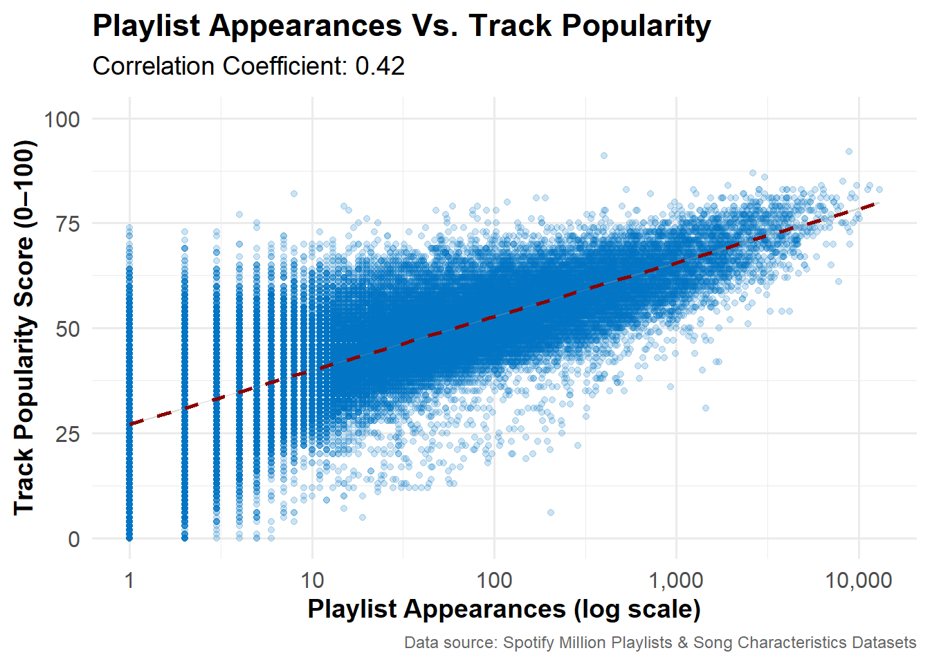
Popularity Score Vs. Number of Playlist Appearances

The figures below show that there is a moderate positive correlation (r = 0.42) between a track’s popularity score and the number of times it appears in user-generated playlists. While tracks that are included in more playlists tend to have higher popularity scores, the variation in the data indicates that playlist appearances do not fully determine track popularity.

Code

# playlist appearances
playlist_appearances <- tidy_songs |>
  distinct(track_id, playlist_id) |>
  count(track_id, name = "playlist_appearances")

# track popularity
popularity <- tidy_songs |>
  select(track_id, track_name, popularity) |>
  distinct()

# combine playlist appearances and popularity 
pop_summary <- left_join(playlist_appearances, popularity, by = "track_id") 

# correlation
corr <- cor(pop_summary$playlist_appearances, pop_summary$popularity, use = "complete.obs")

# display correlation
tibble::tibble(
  Metric = "Playlist Appearances vs. Popularity",
  Correlation = round(corr, 3)) |>
  kbl(caption = "<b>Correlation Between Playlist Appearances and Popularity<b>")|>
  kable_styling(bootstrap_options = c("striped", "hover", "condensed"))

**Correlation Between Playlist Appearances and Popularity**
Metric	Correlation
Playlist Appearances vs. Popularity	0.422

Code

# plot popularity vs playlist appearances
ggplot(pop_summary, aes(x = playlist_appearances, y = popularity)) +
  geom_point(alpha = 0.2, size =1.5, color = "#0073C2FF") +
  geom_smooth(method = "lm", se = TRUE, color = "darkred", linewidth = 1, linetype="dashed") +
  scale_x_log10(labels = scales::comma) + 
  coord_cartesian(ylim = c(0, 100)) +
  labs(
    title = "Playlist Appearances Vs. Track Popularity",
    subtitle = paste0("Correlation Coefficient: ", round(corr, 2)),
    x = "Playlist Appearances (log scale)",
    y = "Track Popularity Score (0–100)",
    caption = "Data source: Spotify Million Playlists & Song Characteristics Datasets") +
  theme_minimal(base_size = 14) +
  theme(
    plot.title = element_text(face = "bold"),
    plot.subtitle = element_text(margin = margin(b = 10)),
    plot.caption = element_text(size = 9, color = "gray40"),
    axis.text = element_text(size = 12),
    axis.title = element_text(size=14, face = "bold")
  )

To identify the common features of popular songs, I created a subset of the combined ‘tidy songs’ data filtered by popularity scores. The threshold for determining whether a song is popular or not-quite popular is somewhat arbitrary. For all subsequent analyses, I am using the 90th percentile popularity score as the threshold. In other words, ‘popular songs’ are defined as those in the top 10% of popularity. For this data, these are all songs with popularity scores of 77 or above. The ‘popular songs’ subset has 839,145 distinct tracks.

Code

# set popularity threshold: 90th percentile popularity score
popularity_threshold <- quantile(tidy_songs$popularity, 0.90, na.rm = TRUE)

# create popular songs data subset
popular_songs <- tidy_songs |>
  filter(popularity >= popularity_threshold)

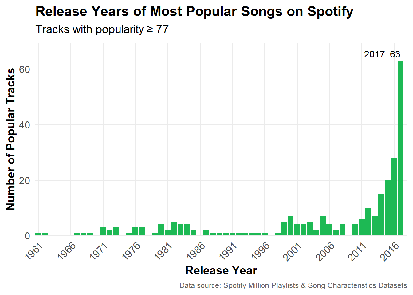
When Were the Most Popular Songs Released?

This figure shows the number of popular songs (as defined by a popularity score of 77 or above) released each year. There is a noticeable upward trend after 2010, peaking in 2017 with 63 popular songs.

The upward trend since 2010 can partly be explained by the growth of Spotify’s platform during this period. The song popularity scores mirror the increase in Spotify’s streaming catalog and user base over the years. Users also tend to listen to and rate recently released songs more than earlier ones, creating a recency bias which can skew the results and explain the long tail of the distribution.

Code

# popular songs by year
popular_songs_yr <- popular_songs |>
  distinct(track_id, .keep_all = TRUE) |>  
  count(year, sort = TRUE)

# year with most popular songs
top_year <- popular_songs_yr |> slice_max(n, n = 1)

# plot of popular songs by release year
ggplot(popular_songs_yr, aes(x = year, y = n)) +
  geom_col(fill = "#1DB954") +
  geom_text(
    data = top_year,
    aes(label = paste0(year, ": ", n)),
    vjust = -0.5,
    hjust = 1,
    color = "black",
    size = 4) +
  scale_x_continuous(
    breaks = seq(min(popular_songs_yr$year), max(popular_songs_yr$year), by = 5),
    minor_breaks = NULL,
    expand = expansion(mult = c(0, 0.01))) +
  scale_y_continuous(
    labels = scales::comma,
    expand = expansion(mult = c(0, 0.1))) +
  labs(
    title = "Release Years of Most Popular Songs on Spotify",
    subtitle = paste0("Tracks with popularity ≥ ", round(popularity_threshold, 1)),
    x = "Release Year",
    y = "Number of Popular Tracks",
    caption = "Data source: Spotify Million Playlists & Song Characteristics Datasets") +
  theme_minimal(base_size = 14) +
  theme(
    plot.title = element_text(face = "bold"),
    plot.subtitle = element_text(margin = margin(b = 10)),
    plot.caption = element_text(size = 9, color = "gray40"),
    axis.text = element_text(size = 12),
    axis.title = element_text(size=14, face = "bold"),
    axis.text.x = element_text(angle = 45, hjust = 1))

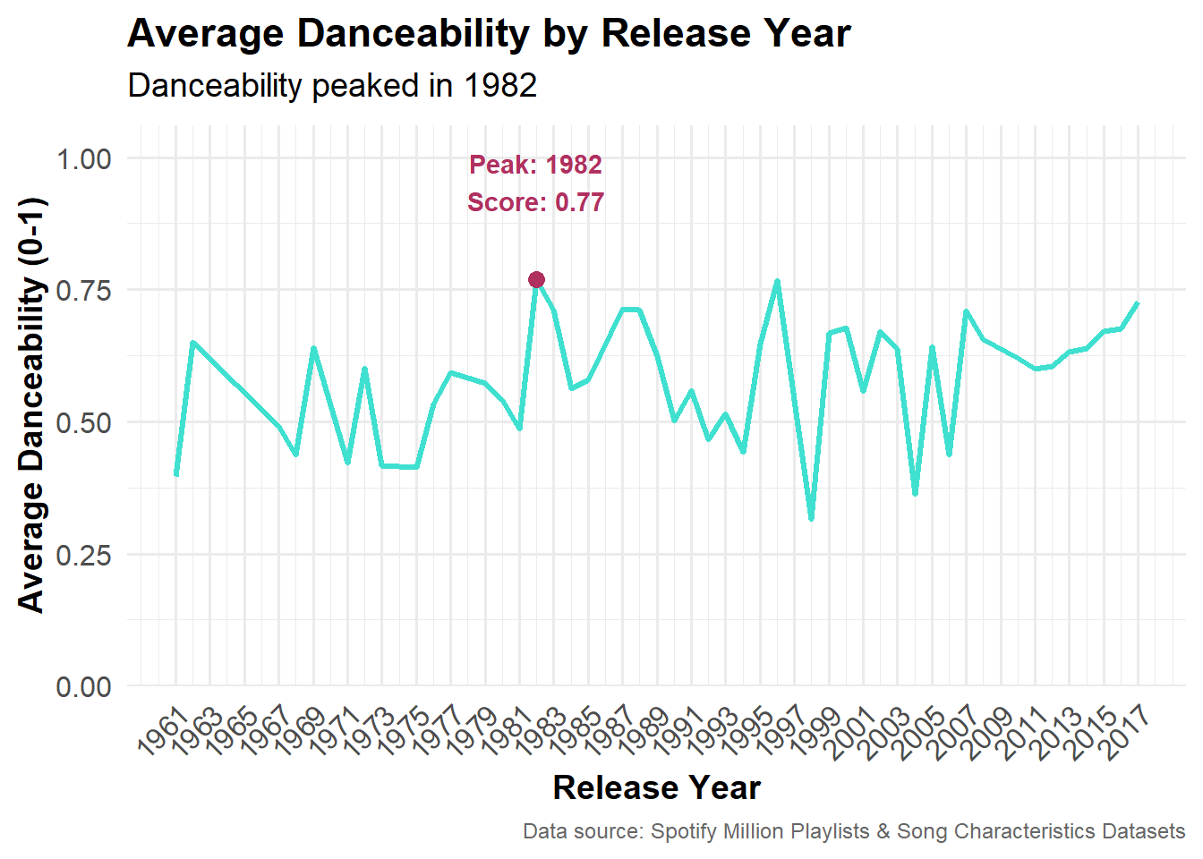
When Did Danceability Peak?

This graph looks at the average “danceability” score of popular songs released each year. The danceability peaked in 1982, with a score of 0.77 (on a scale of 0 to 1). The data also shows a second peak in 1996.

Code

# average danceability by year
dance_by_year <- popular_songs |>
  group_by(year) |>
  summarise(avg_danceability = mean(danceability), .groups = "drop")
# peak year
peak_year <- dance_by_year |>
  filter(avg_danceability == max(avg_danceability))
# plot danceability over years
ggplot(dance_by_year, aes(x = year, y = avg_danceability)) +
  geom_line(color = "turquoise", linewidth = 1.2) +
  geom_point(data = peak_year, 
             aes(x = year, y = avg_danceability), color = "maroon", size = 3) +
  geom_text(data = peak_year, 
            aes(x = year, y = avg_danceability, 
                label = paste0("Peak: ", year, "\nScore: ", round(avg_danceability, 2))), 
            vjust = -1.2, fontface = "bold", color = "maroon") +
  scale_y_continuous(limits = c(0, 1), expand = expansion(mult = c(0, 0.06))) +
  scale_x_continuous(breaks = seq(min(dance_by_year$year), max(dance_by_year$year), by = 2)) +
  labs(
    title = "Average Danceability by Release Year",
    subtitle = paste("Danceability peaked in", peak_year$year),
    x = "Release Year",
    y = "Average Danceability (0-1)",
    caption = "Data source: Spotify Million Playlists & Song Characteristics Datasets") +
  theme_minimal(base_size = 14) +
  theme(
    plot.title = element_text(face = "bold"),
    plot.subtitle = element_text(margin = margin(b = 10)),
    plot.caption = element_text(size = 9, color = "gray40"),
    axis.text = element_text(size = 12),
    axis.title = element_text(size=14, face = "bold"),
    axis.text.x = element_text(angle = 45, hjust = 1))

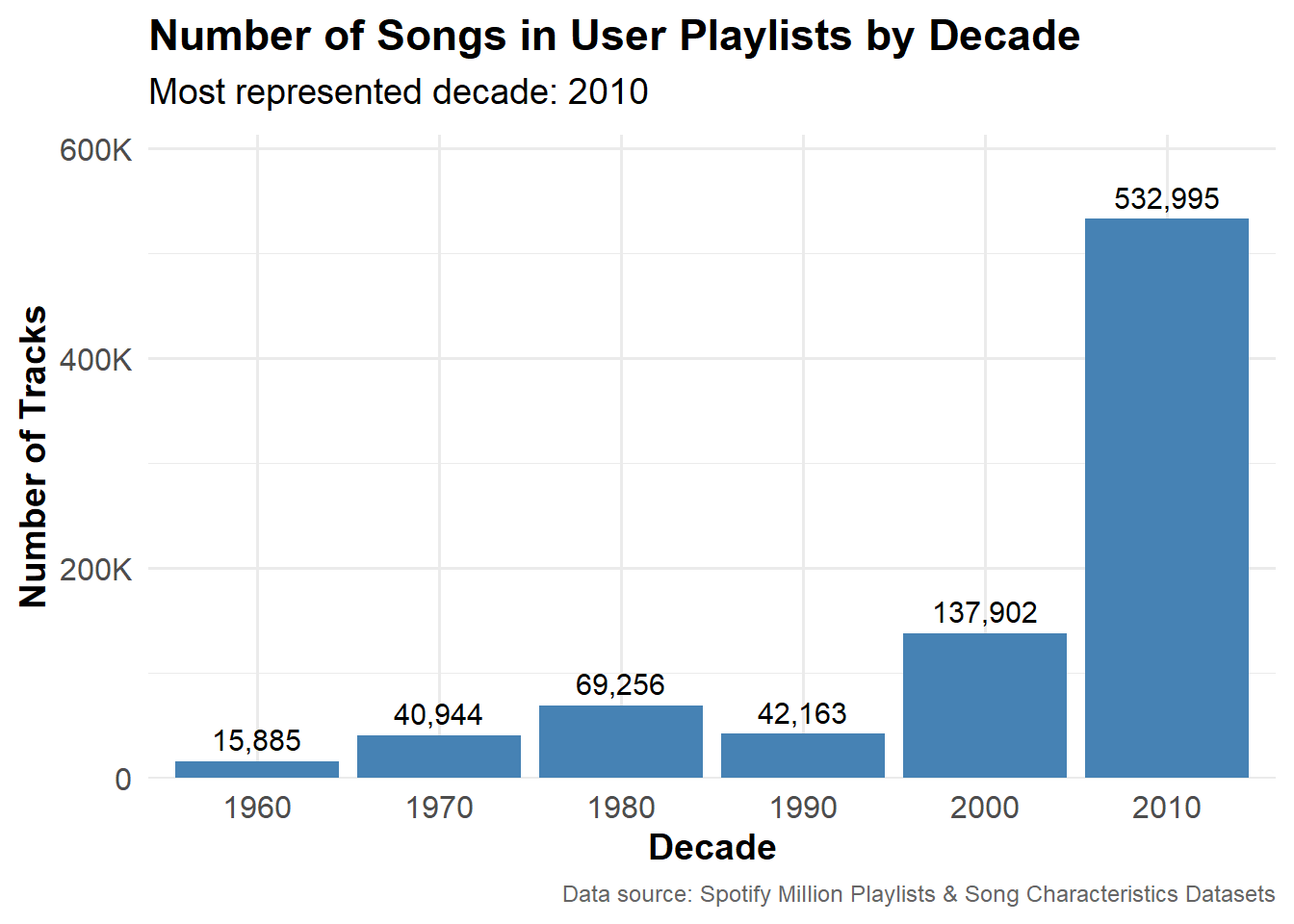
Decade Most Represented in User Playlists

Grouping the number of popular songs (popularity ≥ 77) in user-generated playlists by decade of release shows that the 2010s dominate user playlists with over half a million tracks. This mirrors the upward trend in the number of popular songs released each year. Both trends reflect the growth of Spotify over time and a recency bias in users’ behavior.

Code

# number of popular songs by decade
decade <- popular_songs |>
  mutate(decade = (year %/% 10) * 10) |>
  count(decade, sort = TRUE) 

# most represented decade
most_represented_decade <- decade |> 
  slice_max(n, n = 1)

# plot
ggplot(decade, aes(x = factor(decade), y = n)) +
  geom_col(fill = "steelblue") +
  geom_text(aes(label = comma(n)), vjust = -0.5, size = 4) +
  scale_y_continuous(
    labels = label_number(scale_cut = scales::cut_short_scale()),
    expand = expansion(mult = c(0, 0.15))) + 
  labs(
    title = "Number of Songs in User Playlists by Decade",
    subtitle = paste("Most represented decade:", most_represented_decade$decade),
    x = "Decade",
    y = "Number of Tracks",
    caption = "Data source: Spotify Million Playlists & Song Characteristics Datasets") +
  theme_minimal(base_size = 14) +
  theme(
    plot.title = element_text(face = "bold"),
    plot.subtitle = element_text(margin = margin(b = 10)),
    plot.caption = element_text(size = 9, color = "gray40"),
    axis.text = element_text(size = 12),
    axis.title = element_text(size=14, face = "bold"))

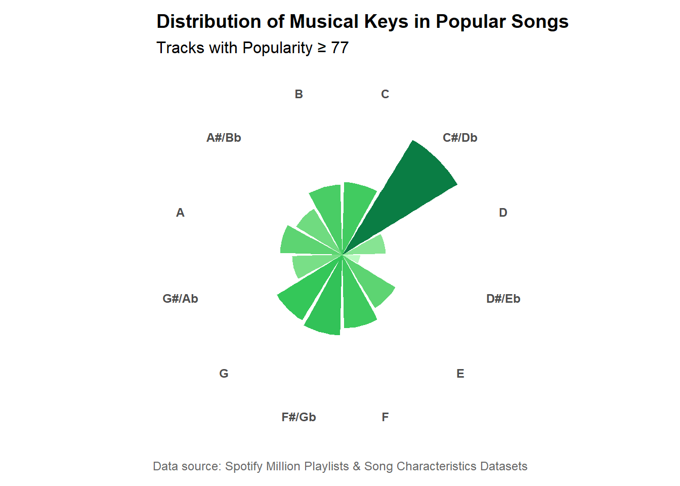
Musical Key Frequency Among Popular Songs

The most common musical key among popular songs (popularity ≥ 77) in user playlists is C♯/D♭, which is surprising considering its difficulty. Musicians generally prefer simpler keys like C, D, and G that are playable on both keyboard and guitar. Due to the way keys are arranged, C♯/D♭ does not play naturally or easily on any instrument.

The results are likely due to several factors:

Sample size and data bias: in addition to the original Spotify data exports not being comprehensive or representative, the ‘popular songs’ subset used here can be skewed if a few very popular tracks are in C♯/D♭.
There could be key detection errors in Spotify’s algorithms.
The data is heavily skewed towards more recent years, and modern popular music is highly auto-tuned and processed. Vocals and instruments are often shifted sharper to sound more bright or sleek for radio and streaming.

In this sense, the key frequency results could actually be pointing towards the dominance of autotuning and post production processing in modern popular music.

Code

# number of songs by key
key_counts <- popular_songs |>
  count(key, sort = FALSE)

# convert key numbers to labels
key_notes <- c("C", "C#/Db", "D", "D#/Eb", "E", "F", 
               "F#/Gb", "G", "G#/Ab", "A", "A#/Bb", "B")
key_counts <- key_counts |>
  mutate(key_label = factor(key_notes[key + 1], levels = key_notes))

# plot
ggplot(key_counts, aes(x = key_label, y = n, fill = n)) +
  geom_col(show.legend = FALSE) +
  coord_polar() +
  scale_fill_gradientn(colors = c("#b9fbc0", "#34c759", "#0a7d44")) +
  expand_limits(y = max(key_counts$n) * 1.1) +
  labs(
    title = "Distribution of Musical Keys in Popular Songs",
    subtitle = paste0("Tracks with Popularity ≥ ", popularity_threshold),
    caption = "Data source: Spotify Million Playlists & Song Characteristics Datasets",
    x = NULL,
    y = NULL
) +
theme_minimal(base_size = 14) +
theme(
  axis.text.y = element_blank(),
  axis.text.x = element_text(size = 9, face = "bold"),
  panel.grid.major = element_blank(),
  panel.grid.minor = element_blank(),
  plot.title = element_text(face = "bold", size = 14),
  plot.subtitle = element_text(size = 12, margin = margin(b = 10)),
  plot.caption = element_text(size = 9, color = "gray40"),
  plot.margin = margin(10, 10, 10, 10))

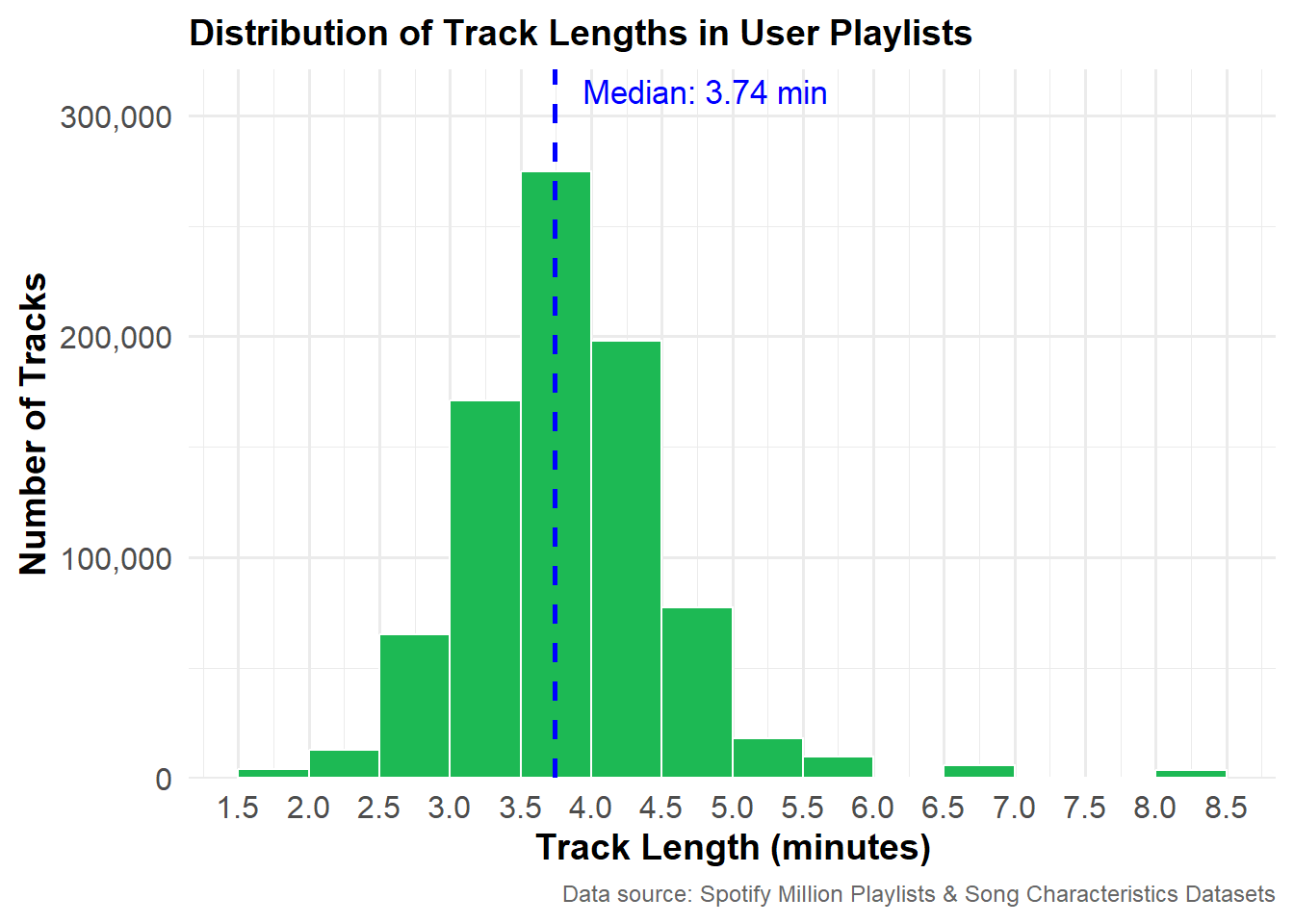
Most Popular Track Lengths In User Playlists

The plot below shows the most popular track lengths in user playlists. The majority of tracks are between 3 and 4.5 minutes long, and the median track length is 3.74 minutes. Tracks shorter than 2.5 minutes and longer than 5.5 minutes are relatively rare.

Code

# convert track duration to minutes
track_lengths <- popular_songs |>
  mutate(duration_min = duration / 60000)  

# median track length
median_length <- median(track_lengths$duration_min, na.rm = TRUE)

# plot
ggplot(track_lengths, aes(x = duration_min)) +
  geom_histogram(binwidth = 0.5, fill = "#1DB954", color = "white", boundary = 0) +
  geom_vline(xintercept = median_length, color = "blue", linetype = "dashed", linewidth = 1) +
  annotate("text",
           x = median_length + 0.2,
           y = 300000,
           label = paste0("Median: ", round(median_length, 2), " min"),
           hjust = 0, vjust = -0.5,
           color = "blue", size = 4.5) +
  scale_x_continuous(breaks = seq(0, 10, by = 0.5)) +
  scale_y_continuous(labels = comma, expand = expansion(mult = c(0, 0.07))) +
  labs(
    title = "Distribution of Track Lengths in User Playlists",
    #subtitle = "Dashed line shows median track length",
    x = "Track Length (minutes)",
    y = "Number of Tracks",
    caption = "Data source: Spotify Million Playlists & Song Characteristics Datasets") +
  theme_minimal(base_size = 14) +
  theme(
    plot.title = element_text(face = "bold", size = 14),
    plot.subtitle = element_text(margin = margin(b = 10)),
    plot.caption = element_text(size = 9, color = "gray40"),
    axis.text = element_text(size = 12),
    axis.title = element_text(size=14, face = "bold"))

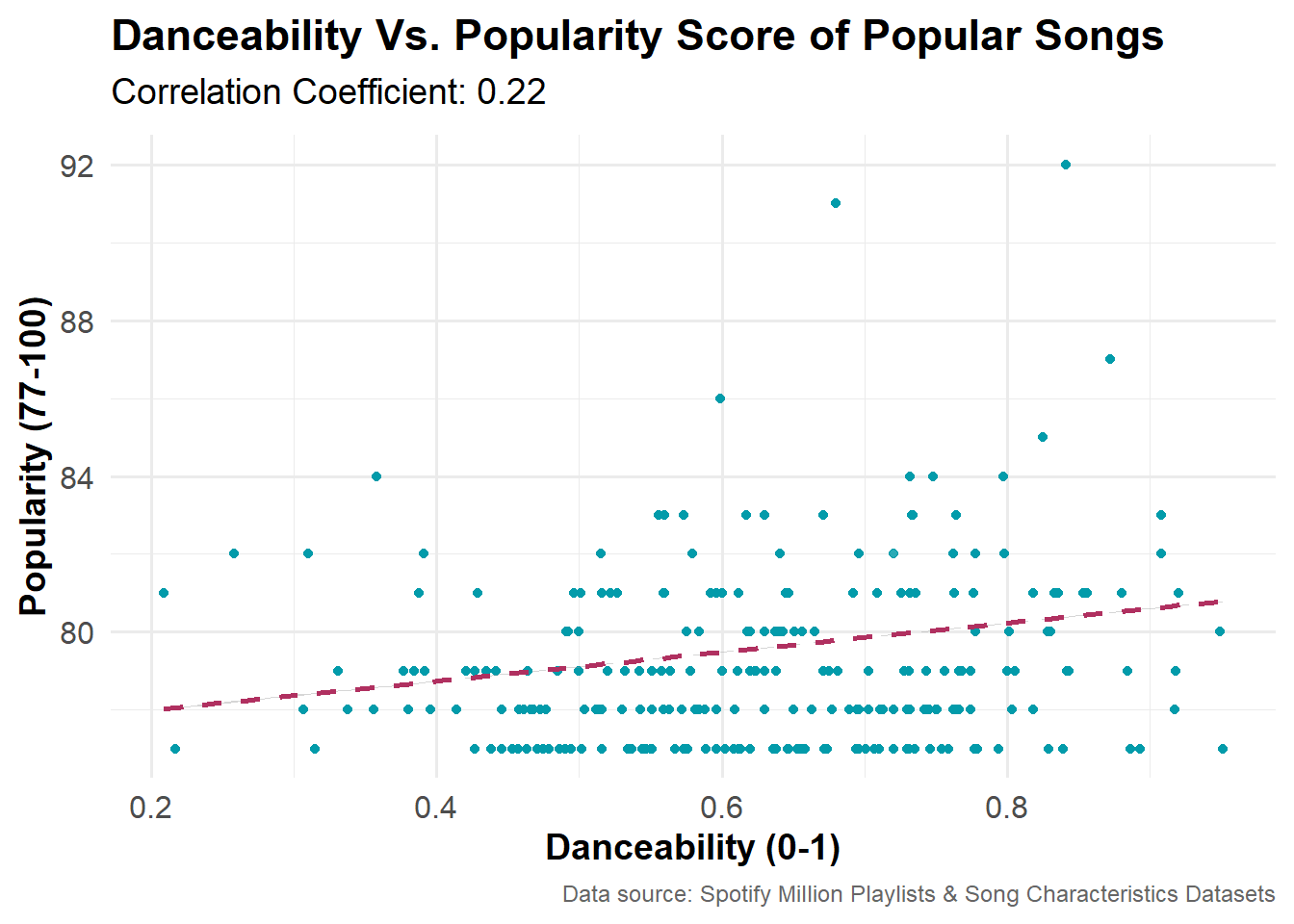
Danceability Vs. Popularity Score of Popular Songs

This scatterplot shows a slight positive relationship between the danceability score of a song (on a scale of 0-1 ) and the popularity score of songs (popularity ≥ 77). The correlation coefficient is 0.22, indicating that songs with high danceability are marginally more popular, but the relationship is not strong. Of course, this subset only contains songs in the top 10% of popularity, so there is less variation in the data to explain.

Code

# correlation between danceability and popularity among popular songs
cor1 <- cor(popular_songs$danceability, popular_songs$popularity)

# plot
ggplot(popular_songs, aes(x = danceability, y = popularity)) +
  geom_point(alpha = 0.2, size =1.5, color = "#0099a8") +
  geom_smooth(method = "lm", se = TRUE, color = "maroon", linewidth = 1, linetype = "dashed") +
  labs(
    title = "Danceability Vs. Popularity Score of Popular Songs",
    subtitle = paste0("Correlation Coefficient: ", round(cor1, 2)),
    x = "Danceability (0-1)",
    y = "Popularity (77-100)",
    caption = "Data source: Spotify Million Playlists & Song Characteristics Datasets") +
  theme_minimal(base_size = 14) +
  theme(
    plot.title = element_text(face = "bold"),
    plot.subtitle = element_text(margin = margin(b = 10)),
    plot.caption = element_text(size = 9, color = "gray40"),
    axis.text = element_text(size = 12),
    axis.title = element_text(size=14, face = "bold"))

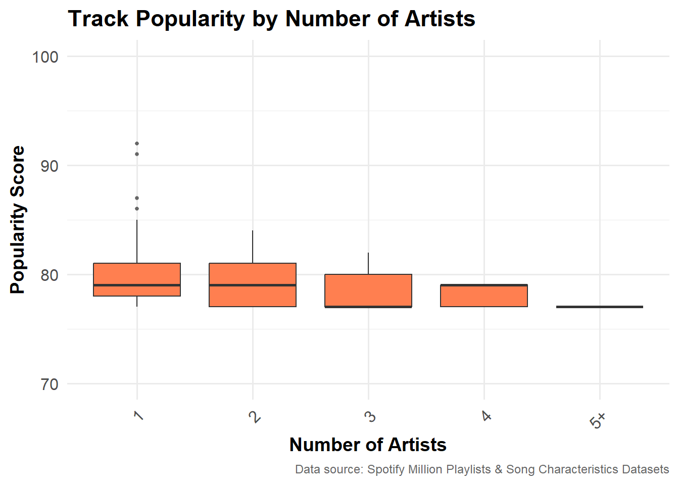
Relationship Between Number of Artists and Popularity

Do songs with more artist collaborations tend to be more popular? Or do solo tracks dominate popularity? This graph shows the distribution of popularity scores by number of artists in the ‘popular songs’ data (popularity ≥ 77). Tracks with 1 or 2 artists are the most common and have slightly higher median popularity compared to tracks with more artists.

Code

# mutate num_artists variable
popular_songs <- popular_songs |>
  mutate(num_artists_grouped = ifelse(num_artists >= 5, "5+", as.character(num_artists)))

# boxplot of popularity score by number of artists
ggplot(popular_songs, aes(x = factor(num_artists_grouped), y = popularity)) +
  geom_boxplot(fill = "coral", outlier.color = "gray40", outlier.size = 1) +
  coord_cartesian(ylim = c(70, 100)) +
  labs(
    title = "Track Popularity by Number of Artists",
    x = "Number of Artists",
    y = "Popularity Score",
    caption = "Data source: Spotify Million Playlists & Song Characteristics Datasets") +
  theme_minimal(base_size = 14) +
  theme(
    plot.title = element_text(face = "bold"),
    plot.subtitle = element_text(margin = margin(b = 10)),
    plot.caption = element_text(size = 9, color = "gray40"),
    axis.text = element_text(size = 12),
    axis.text.x = element_text(angle = 45, hjust = 1),
    axis.title = element_text(size=14, face = "bold"))

Building a Playlist From Anchor Songs

To build our playlist, we pick an “anchor song” and then find songs that fit well with this song using various heuristics, or ‘rules of thumb’. The Spotify data used here does not include song genre, theme, or any artist information besides their name, so the rules of thumb will have to focus on songs co-occurring on the same playlists, released within the same time period, and having similar metrics such as key, tempo, danceability, etc.

The specific heuristics used in this analysis are:

Playlist co-occurrence: songs that commonly appear on the same playlists as the anchor song.
Musical Similarity: songs that are in the same key and have a similar tempo.
Same Artist: songs released by the same artist.
Same Release Year and Characteristics: songs released in the same year and with similar levels of danceability, acousticness, etc.
Same Release Decade, Danceability, and Energy: songs released within the same decade and with similar levels of danceability and energy.

The code below uses ‘Toxic’ by Britney Spears as the anchor song. I implemented the five heurestics mentioned above to identify related songs. As ‘Toxic’ is a very popular song, I only counted songs that co-occurred at least 10 times on the same playlists. The results from all heuristics were combined into an initial candidate list. This initial candidate list was too broad, so it was filtered again by decade and by key metrics such as danceability, energy, popularity, and tempo. The resulting shorter candidate list was then scored, ranked, and randomly sampled to get the final playlist candidate list of 30 tracks.

Code

# set anchor song: 'Toxic' by Britney Spears
anchor_id <- "6I9VzXrHxO9rA9A5euc8Ak"
anchor_song <- tidy_songs |> filter(track_id == anchor_id)

# playlists containing the anchor song
anchor_playlists <- tidy_songs |>
  filter(track_id == anchor_id) |>
  distinct(playlist_id)

# other songs from the same playlists (filtered to those appearing at least thrice)
common_songs <- tidy_songs |>
  filter(playlist_id %in% anchor_playlists$playlist_id,
         track_id != anchor_id) |>
  count(track_id, sort = TRUE) |>
  filter(n >= 10) |>   # <--- ADD THIS LINE HERE
  left_join(
    tidy_songs |> 
      select(track_id, track_name, artist_name, popularity, year, danceability, tempo, key, mode, energy, acousticness, valence),
    by = "track_id"
  ) |>
  distinct(track_id, .keep_all = TRUE)

# songs with same key and similar tempo (+/-5bpm)
same_key_tempo <- tidy_songs |>
  filter(
    key == anchor_song$key,
    abs(tempo - anchor_song$tempo) <= 10,
    track_id != anchor_id) |>
  distinct(track_id, .keep_all = TRUE) |>
  select(track_id, track_name, artist_name, popularity, year, danceability, tempo, key, mode, energy, acousticness, valence)

# songs from the same artist
same_artist_songs <- tidy_songs |>
  filter(artist_name %in% anchor_song$artist_name,
         track_id != anchor_id)|>
  distinct(track_id, .keep_all = TRUE) |>
  select(track_id, track_name, artist_name, popularity, year, danceability, tempo, key, mode, energy, acousticness, valence)

# songs released in same year with similar danceability, energy, acousticness, valence
similar_features <- tidy_songs |>
  filter(
    year == anchor_song$year[1],  
    abs(danceability - anchor_song$danceability[1]) < 0.1,
    abs(energy - anchor_song$energy[1]) < 0.1,
    abs(acousticness - anchor_song$acousticness[1]) < 0.1,
    abs(valence - anchor_song$valence[1]) < 0.1,
    track_id != anchor_id)|>
  distinct(track_id, .keep_all = TRUE) |>
  select(track_id, track_name, artist_name, popularity, year, danceability, tempo, key, mode, energy, acousticness, valence)
  
# songs released in same decade with similar energy and danceability
# get anchor decade
anchor_decade <- (anchor_song$year %/% 10) * 10
# find songs with same vibes
vibe_matches <- tidy_songs |>
  filter(
    (year %/% 10) * 10 == anchor_decade,
    abs(danceability - anchor_song$danceability[1]) < 0.1,
    abs(energy - anchor_song$energy[1]) < 0.1,
    track_id != anchor_id)|>
  distinct(track_id, .keep_all = TRUE) |>
  select(track_id, track_name, artist_name, popularity, year, danceability, tempo, key, mode, energy, acousticness, valence)

# combine all 5 heuristics and filter by same decade to get initial list of candidates
initial_candidates <- bind_rows(
  common_songs,
  same_key_tempo,
  same_artist_songs,
  similar_features,
  vibe_matches
) |>
  distinct(track_id, .keep_all = TRUE) 

# filter initial candidates list
strong_candidates <- initial_candidates |>
  filter(
    (year %/% 10) * 10 == anchor_decade,
    danceability >= 0.6,
    energy >= 0.5,
    tempo >= 95,
    popularity >= 50,
    acousticness < 0.5) 

# score candidates
top_scored_candidates <- strong_candidates |>
  mutate(
    score = danceability * 0.4 +
            energy * 0.3 +
            popularity/100 * 0.3
  ) |>
  arrange(desc(score)) |>
  slice_head(n = 100)

# randomly sample 30 tracks from top 100
set.seed(123)
sampled_candidates <- top_scored_candidates |>
  slice_sample(n = 30)

The Ultimate 2000s Dance Party Playlist

The table below shows the final playlist, curated to embrace the 2000s dance party vibes. It starts out strong with huge hits from Shakira, Nina Sky, and Britney, the Queens of 2000s dance floors. It ramps up and builds energy and intensity with tracks from Flo Rida, T.I., LMFAO. Then, it mellows just slightly before ending strong with “Overnight Party” and “Smack That.”

Code

# selected tracks
selected_tracks <- c(
  "Hips Don't Lie",
  "Move Ya Body",
  "She Wolf",
  "I'm a Slave 4 U",
  "Low (feat T-Pain) - Feat T-Pain Album Version",
  "Bring Em Out",
  "Shots",
  "Ella",
  "Wipe Me Down (feat. Foxx, Webbie & Lil Boosie) - Remix",
  "Still Tippin' (feat. Slim Thug and Paul Wall) - featuring Slim Thug and Paul Wall",
  "Overnight Celebrity",
  "Smack That - Dirty"
)

# filter sampled candidates to only include selected tracks
final_playlist <- sampled_candidates |>
  filter(track_name %in% selected_tracks) |>
  mutate(order = match(track_name, selected_tracks)) |>
  arrange(order) |> 
  select(order, track_name, artist_name, popularity, year, danceability, tempo, energy, valence)

# display playlist in spotify green
 final_playlist |>
  kable("html", escape = FALSE, align = "c", col.names = c(
    "Order", "Track Name", "Artist", "Popularity", "Year", 
    "Danceability", "Tempo (BPM)", "Energy", "Valence"
  )) |>
  kable_styling(bootstrap_options = c("striped", "hover", "condensed", "responsive"), 
                full_width = FALSE, 
                position = "center",
                font_size = 14) |>
  row_spec(0, bold = TRUE, color = "white", background = "#4CAF50") |> 
  column_spec(1, bold = TRUE) |> 
  column_spec(2:9, width = "10em")

Order	Track Name	Artist	Popularity	Year	Danceability	Tempo (BPM)	Energy	Valence
4	I'm a Slave 4 U	Britney Spears	66	2001	0.847	110.027	0.843	0.963
6	Bring Em Out	T.I.	63	2004	0.759	98.579	0.891	0.587
7	Shots	LMFAO	67	2009	0.825	128.016	0.856	0.207
8	Ella	Bebe	61	2004	0.843	118.006	0.797	0.866
9	Wipe Me Down (feat. Foxx, Webbie & Lil Boosie) - Remix	Boosie Badazz	60	2007	0.836	165.091	0.906	0.718
12	Smack That - Dirty	Akon	70	2006	0.939	118.978	0.742	0.924

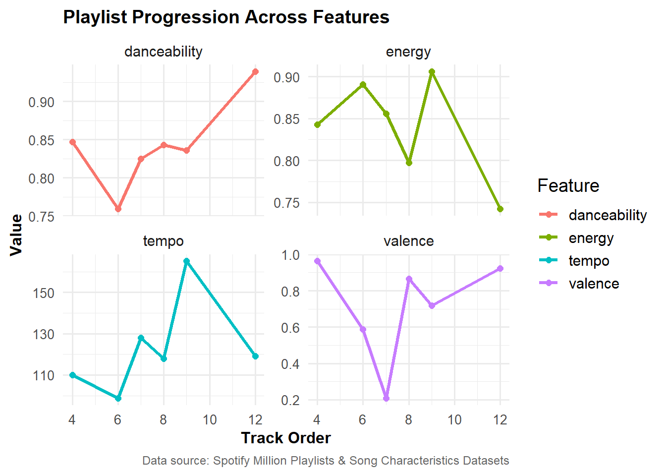
This playlist was optimized for dancing. The danceability starts and stays fairly high throughout, around 0.8-0.9 (on a scale of 0-1), and ends at its peak. The energy and tempo are also high, with some dips around track 4-6, before picking back up after track 7. The tempo peaks at track 9 before slowly winding down. The valence, or emotion/mood, starts high, dips sharply around tracks 5-6 before rising again, creating some emotional contrast and a feel-good closure.

Code

final_playlist_long <- final_playlist |> 
  pivot_longer(cols = c(danceability, energy, tempo, valence),
               names_to = "Feature", values_to = "Value")

ggplot(final_playlist_long, aes(x = order, y = Value, color = Feature)) +
  geom_line(size = 1.2) +
  geom_point(size = 2) +
  facet_wrap(~ Feature, scales = "free_y") +
  theme_minimal() +
  labs(title = "Playlist Progression Across Features", 
       x = "Track Order", 
       y = "Value",
       caption = "Data source: Spotify Million Playlists & Song Characteristics Datasets") +
  theme_minimal(base_size = 14) +
  theme(
    plot.title = element_text(face = "bold", size=14),
    plot.subtitle = element_text(margin = margin(b = 10)),
    plot.caption = element_text(size = 9, color = "gray40"),
    axis.text = element_text(size = 10),
    axis.title = element_text(size=12, face = "bold"))

Warning: Using `size` aesthetic for lines was deprecated in ggplot2 3.4.0.
ℹ Please use `linewidth` instead.